Activity 19 Restoration of blurred images

The main objective of this activity is to restore an image corrupted by a known degradation function and an additive noise using Mean square error (Weiner) filtering.
In order to perform this, we first choose a clean grayscale image containing some texts within. The chosen image is shown in Figure 1. This image was then degraded by adding a Gaussian noise with it. The discussion about this noise model has been stated in the previous activity.
To perform the restoration, a simple model adapted from the handout [1] is displayed in figure 2. The image is degraded by convolving the degradation function h(x,y) with the image f(x,y) and adding the Gaussian noise (x,y). Note that this is in spatial domain. In order to transform this to the frequency domain, we take the Fourier transform of the terms and apply equation 2 in the handout, given by:

where capital letters correspond to the Fourier transform of the functions.

Figure 1. Clean image

Figure 2. Model of image degradation and restoration.

If we assume that the image is blurred by a linear motion between the sensor and the image during the acquisition, the image then undergoes a planar displacement in the x and y direction which varies through time t. In order to obtain to total exposure at any point of the recording medium, the integral of the instantaneous exposure is taken over the time interval for which the imaging shutter is opened. And if the opening and closing of the shutter occurs instantaneously, we can isolate the image motion and arrive at the blurred image using the formula:

where T is the exposure time. This can also be expressed in the frequency domain which is equivalent to:

The degradation function H is estimated using the following expression

Note that the variables a and b correspond to the total distance from which the image is displaced in the x and y direction.

In order to employ Weiner filtering, we treat the the image and the noise as random processes and try to estimatesuch that its mean square error with the original image f is small. This is performed mathematically by using the the equations:

where

.

Alternatively, the expression for F above can be approximated by the equation:

where K is a constant. This is particularly used when we are dealing with spectral white noise such that the spectrum is constant.

By varying the parameters a b and T, we apply Gaussian noise and degrade the image. The results for this degradation process are shown in Figure2. Using the last two expressions for , we try to restore these blurred images and the are shown in Figures 3 and 4.

Figure 2. Degradation of the image using different values of a, b, and T

Upon increasing the values of a and b, image becomes more blurry. This is reasonable since upon increasing the distance for which the image is displaced along the x and y axis with respect to the recording medium, lesser the information about the image can be generated. And it is seen that at a=b= 0.1, most of the information regarding the image is lost.

Figure 3. Restoration of the image using Weiner Filtering

From the figure above, the quality of the degraded image was improved, although it was not totally recovered. And comparing the images before and after applying Weiner flitering, we can observe that some of the information regarding the original image were restored. However, among the four sets of images, the restoration for a=b=0.1 is poorest.

Figure 4. Restoration of the image using Weiner Filtering equation 2 for different K, a, b, and T.

After using the second equation for the Weiner filtering and using different values for K (0.005-0.01 with 0.001 interval), restoration of some information in the image was done. However, if we compared the result with Figure 3, it can be seen that richer image quality is obtained in the first expression. And after varying K, no significant difference was observed.

In this activity, I was able to restore the degraded image corrupted with a degradation function and a Gaussian noise model so I am giving myself a grade of 10.

Reference:
" Restoration of blurred images", Activity 18 Handout, Applied Physics 186.

Activity 18 Noise model and basic image restoration

In this activity, we try to demonstrate the different types of noise and image restoration techniques. Similar to image enhancement technique, this method aims to improve the quality of images surrounded with noise. However, this technique is more of object type as compared to image enhancement technique which is subjective in nature.

The image below shows the clean image composed of three grayscale values. The corresponding probability distribution function (PDF) of the gray levels of the clean image is also shown together with the image.

Figure 1. Clean image and its PDF

The different noise models that are applied to the image above are as follows:

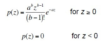
1. Gaussian noise
This model is also known as the normal noise model from which the PDF is given by:

where z is the gray level value, is the average, and is the standard deviation.

2. Gamma/Erlang noise
This model has a PDF equal to:

and the mean and variance are given by:

3. Exponential noise model
For this model, the PDF is given as:

and the mean and variance of the density are:

4. Rayleigh noise model
The PDF of the Rayleigh noise model is given by:

and the mean and variance are determine using the equations:

5. Uniform noise model
To determine the PDF, mean, and variance of this model, the following equations are used.

6. Impulse (Salt and Pepper) noise model
The PDF of this model is:

These noise models were simulated using the "grand" function available in Scilab programming language. The effect of the different noise model on the clean image is investigated and shown in Figure 2. Notice from the PDF of the different noise models that the graylevels of the image which were supposedly consisting of only three values become broad and occupied other graylevel values. Depending on the parameters of the noise model, the width of the broadening can be varied. From Figure 2, it can also be noticed that after adding a uniform noise to the image, the graylevels become very large in range such that the values from ~125 to 255 were covered.

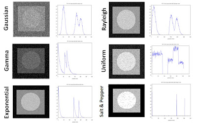
Figure 2. Different noise models applied to the clean image

In order to improve the quality of the degraded image brought by the added noise, spatial filtering method is employed. The different filters that are utilized in this activity are as follows.

Arithmetic Mean Filter (AMF)
In this method, a window S_xy with dimensions m x n and centered at point (x,y) from the corrupted image g(x,y) is selected and the average values of g(x,y) in the area of the window is computed. This can be expressed mathematically as:

where f(x,y) is the restored image.

Geometric Mean Filter (GMF)
This filter is used by implementing the following formula for computing the restore image f(x,y).

Harmonic Mean Filter (HMF)

To restore the corrupted image brought by the addition of noise, this filter is employed by following the formula:

Contraharmonic Mean Filter (CMF)
This filter works by using the expression:

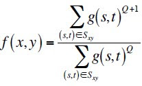
where Q is the order of the filter. Different values of Q yields the removal of either salt or pepper noise and it cannot eliminate both the salt and pepper at the same time.

By implementing the formula given for every filter, the corrupted images after adding the different noise models were restored and shown in the figures below together with the PDF of the restored images.

Figure 3. Restoration of image with Gaussian noise

Figure 4. PDF of the restored image contaminated with Gaussian noise

From the restored images and their corresponding PDF, Gaussian noise was partially eliminated. From the originally very noisy image, the different filters showed an enhancement of the image quality. By observing the PDF of the restored images after using the 4 filters discussed above, it can be seen that the graylevels of the image became narrower in range. However, the initially white part of the image was converted to some other grays values.

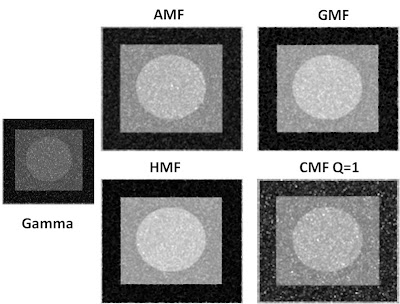
Figure 5. Restoration of image with Gamma noise

Figure 6. PDF of the restored image contaminated with Gamma noise

After applying the different filters on the image contaminated with Gamma noise, the characteristic of the image became better in such a manner that the PDF showed three peaks with graylevel values close to the original image. Among the four filters, contraharmonic filter exhibit the worst restoration because the corresponding PDF of the image which was treated still showed a broad graylevel values. This can be further improved by trying other values for Q.

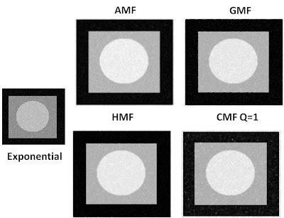
Figure 7. Restoration of image with Exponential noise

Figure 8. PDF of the restored image contaminated with Exponential noise

For the exponential noise that was added to the image, the four filters were shown to be effective in restoring the originally uncontaminated image. However, observing the PDF of the image treated with an arithmetic mean filter, there is an appearance of other peaks aside from the three high peaks.

Figure 9. Restoration of image with Uniform noise

Figure 10. PDF of the restored image contaminated with Uniform noise

Figure 11. Restoration of image with Rayleigh noise

Figure 12. PDF of the restored image contaminated with Rayleigh noise

The restoration of the image with uniform and rayleigh noise was also successfully done the four spatial filters. By comparing the PDF of the initially very noisy image when uniform noise is added and the PDF after applying the filter, we can see that there is a large improvement on the quality of the image.

For the salt and pepper noise added to the image, it can be seen that contraharmonic mean filter works best among the four filters. Further investigation was done when this filter is applied for different Q. In order to evaluate the mechanism of the filter for every Q, I used four values of Q, from -2 to +2 with an increment of 1 and applied CMF to the image contaminated with salt and pepper noise. The corresponding images with their PDF are shown in Figures 15 and 16.

Figure 13. Restoration of image with Salt and Pepper noise


Figure 14. PDF of the restored image contaminated with Salt and Pepper noise

Figure 15. Restoration of image contaminated with salt and pepper noise using CMF at different Q.

Figure 16. PDF of the restored image after using CMF at different Q

From the plots above, notice that if Q is negative, salt noise is eliminated while for positive Q, pepper noise is removed.

The different noise model and spatial filters for image restoration are again utilized for another image and the results are shown below.

For this activity, I was able to show the different noise models and their effects on the image as well as the image restoration using the discussed spatial filters. Since the objective of the experiment was met, I give myself a grade of 10.

Reference:

"Noise model and basic image restoration", Applied physics 186 Activity 18 Handout
image: http://www.inhabitat.com/wp-content/uploads/fostergianttower.jpg

Activity 17 Photometric Stereo

As from our previous activities, we know that the brightness of an object highly depends on the amount of light it receives from the source and the reflectance of the object's surface.

Consider the image shown above. The variable P resembles the point at the surface, p(P) is the reflectance, S(P) is the vector from P to the source, n(P) is the normal vector at point P, and r(P) is the distance from P to the source. For a point source, the brightness decreases to 1/r^2 and this proportionality is more clearly seen for a nearby point source, wherein the brightness is given by:

If the light source is at infinity, the light wave approaching the object appears similar to a plane wave, and the brightness becomes:

where S(P) becomes equal for all direction. Finally, for a line source, the brightness decreases proportional to 1/r.

Given a light source shone to an object at different positions, we can reconstruct the 3D shape of the surface of the object. The technique employed for this problem is Photometric Stereo. In this method, we capture multiple images of the surface at different locations and use these images to generate the vectors normal to the surface.


In this activity, we reconstruct the 3D shape of an object which is illuminated by a source from a very far location. We assume that the brightness of the object is proportional to the intensity I captured by the camera at different positions V which are represented by the different images and matrix shown below.

We utilize the I and V values to the equations:

where g corresponds to the product of the reflectance and the normal vector. We solve for this variable in order to determine the surface normal vector n. The next two equation are used for this step.

Since the surface normals are related to the partial derivative of the elevation of the surface f, we can integrate the derivative to finally compute the surface elevation. The equation given below represents the elevation at any point (u,v) .

Following the steps above, f(u,v) was calculated and plotted to arrive at the 3D shape of the object displayed below.

The main objective of this activity which is the reconstruction of the 3D plot of the object was fulfilled so I am giving myself a grade of 10.


Reference:
"Photometric Stereo",Activity 17 Manual in AP 186.

Activity 16 Neural Networks

In this activity, pattern recognition is employed by using neural networks...

Neural network is a computational model that mimics the behavior of the neurons in the brain [1]. It is more advantageous than linear discriminant analysis because it also considers nonlinear systems. It is able to model nonlinear functions containing large variables which make it useful to several applications such as detection of medical phenomena, stock market prediction, credit assignment, monitoring the condition of machinery, and engine machinery [2].

To implement neural network model, I considered 10 sample objects consisting of blue and red dinosaurs as shown in Figure 1. Four feature vectors, namely the red chromaticity value, green chromaticity value, blue chromaticity value, and area were utilized for classification. The area values of the objects were normalized with respect to the highest value so the feature vectors can be correlated with one another. The first five rows of each column correspond to the blue dinosaurs while the last five rows describe the feature vectors of the red dinosaurs. The matrix below shows the arrangement of the training set and the feature vectors. The first, second, third, and fourth columns are designated to red chromaticity value, green chromaticity value, blue chromaticity value, and normalized area, respectively.

Figure 1. Image used for neural network

For this case, I chose the red dinosaurs as my desired class, so the desired output is written such that the class of blue dinosaurs is set to 0 and red dinosaurs to 1. By adopting the code of Mr. Jeric Tugaff for neural network posted in Mr. Cole’s blog [3], the results shown in Figure 2 and 3 were obtained. The number of iterations (T) and learning rate (LR) were varied and their effects to the accuracy of recognition were observed. The values for T were changed from 100 to 500 with an increment of 100, and it was found that more accurate pattern recognition is acquired for higher T, that is, blue-colored dinosaurs resulted to values nearest to 0 and red dinosaurs nearest to 1. Thus, T=500 yield the most accurate pattern recognition ability from the range chosen, and it was utilized for determining the effect of LR to the accuracy of recognition (see Figure 3). LR was varied from 0.1 to 2 and it can be observed that more accurate pattern recognition is attained as the LR is increased. From the range of LR values, LR=2 yielded the highest accuracy for pattern recognition by having values of red dinosaurs closest to 1 and blue dinosaurs closest to 0. However, it cannot be concluded that T=500 and LR=2 are the optimized parameters for acquiring the most accurate pattern recognition ability since we can still extend the range and seek for more combination of LR and T.

Figure 2. Results obtained for different T


Figure 3. Results obtained for different LR

Since I was able to meet the objective of the activity, I give myself a grade of 10. I would like to acknowledge Master and Orly for helping me improve my results.

References:

1. "Neural Networks", Activity 16 Manual.

2. "Neural Networks", Statsoft Inc., http://www.statsoft.com/textbook/stneunet.html#apps.

3. http://cole-ap186.blogspot.com/

Activity 15 Probabilistic Classification

Pattern recognition was performed in the previous activity using the Euclidean distance. Now, we are going to employ Linear Discriminant Analysis (LDA) for classifying members of a certain group. The image from the previous activity are reused for this purpose and is shown in Figure 1. LDA shows that groups can be separated by a linear combination of features that are used to describe the members.

Figure1. Image used for pattern recognition using LDA

Using the object features, the members are assigned to the group with highest conditional probability. This is known as Baye's rule, which helps minimize the total error of classification (TEC). Mathematically, it is expressed as the object belong to group i where

Thus, the probability that the member belongs to group i given a set of data x is determined.

To implement LDA, we form a matrix x consisting of rows of objects and columns of features. For this particular activity, I used the same objects (blue and red dinaosaurs) and same features as the previous activity, that is, r_values and area. From this matrix, the two classes of objects are separated (x1 and x2) with their corresponding features. To visualize this, refer to the equation below.

From x1 and x2, the mean features u1 and u1, and global mean vector are determined which are used to get the mean corrected data x10 and x2o. From these values, the pooled covariance matrix are calculated using the equation

where g is the number of groups ci(r,s) is the covariance of each group. Finally, the discriminant function is solved using the following formula:

The selection of an object to a particular group is by choosing the Fi of the class with higher value. Here, F1 correspond to the class of red dinosaurs while F2 to the blue dinosaurs. Table 1 shows the result after performing LDA.

Table 1. Results obtained after applying LDA

The percentage of correct prediction of the classification is 100%.
For this activity, I am able to apply LDA to classify objects belonging to a certain class. Since I met the objective, I give myself a grade of 10.

References:
http://people.revoledu.com/kardi/tutorial/LDA/
http://www.craftkitsandsupplies.com/images/Foam_Shapes/Foam_Dinosaur_Shapes.jpg

Activity 14 Pattern Recognition

In image processing, it is important to distinguish sets of classes which share common features such as size, shape, color, and others. These sets of features are known as pattern and the process of determining the set of features that will enable the separation of a set into classes in called pattern recognition. In this activity, our task is to apply pattern recognition in images. Careful choice of the class features is important in this activity since it helps simplify our problem.

Mathematically, patterns maybe arranged into ordered sets such as feature vectors. If we let ωj, where j=1, 2, 3, …, W be a set of classes and W the total number of classes, we can define a representative of class ωj such that its mean feature vector is:

where xj is the set of all feature vectors in class ωj and Nj is the number of sampls in ωj. The class membership is determined by classifying an unknown feature vector x to the class whose mean is nearest to it. The Euclidean distance is used for this case and is equal to:

where is the ||y|| = (y^Ty)^1/2 Euclidean norm [1].

The image [2] chosen for this activity is shown in Figure 1. As seen from the figure, the members of the entire class are dinosaurs of different types. From these dinosaurs, two classes are chosen and are shown in Figure 2. The figure consists of 5 blue dinosaurs and 5 red dinosaurs. The first three pictures of each row served as the training sets while the last two are the test objects. The classes are differentiated from each other in terms of color and area. For the first feature in our pattern recognition, the RGB values of each training sets are determined. Then, the normalized chromaticity for red (denoted as r_value) and the mean r_value for the two classes are calculated. For the second feature, i.e. area, the training objects are first converted to binary images (with proper thresholding). Using the code for area calculation in activity 2, the area of each training object and the mean area for each class are obtained. Table 1 shows a summary of the r_value and area for each training object.

Figure 1. Image used for pattern recognition [2]

Figure 2. Selected classes from image



Table 1. r_value and area of the training set.

To clearly see the separation between the two classes using the features selected, the r_values for differentarea of each training object are plotted and is shown in Figure 3. Notice that the separation between the classes is large enough to classify the objects. This signifies that the chosen features are reliable for pattern recognition.

Figure 3. Plot of r_values versus area of the training objects

For the test objects, the r_value and area are also calculated. Using Euclidean distance, test objects are classified as to what class they belong. The computed values and the classifications are shown in Table 2 and the plot of r_values vs. area is shown in Figure 4.

Table 2. Tabulated r_value and area of the test objects and their classifications

Figure 4. Plot of r_values vs. area of the test objects

From this activity, I was able to perform pattern recognition by supplying the right feature of each class and predicting the class from which the test objects belong. I would like to thank Kaye Vergel for that good discussion.

Since I am able to meet the objective of the activity, I give myself a grade of 10.

References:

1. Activity manual for Pattern recognition

2. http://www.craftkitsandsupplies.com/images/Foam_Shapes/Foam_Dinosaur_Shapes.jpg

Preprocessing Text

Extracting information from handwritten texts is one of the problems in image processing. Several steps and methods are usually used in order to get the desired information like the removal of embedded lines and text separation. In this activity, previous knowledge regarding image processing techniques are applied to recognize handwriting from a given text document.

Step by step procedure

• Download the text document and crop a certain portion which shows texts together with the horizontal lines. (See Figure 1)
  
• Make a filter mask by taking the Fourier transform of the cropped image and modifying it using Gimp to remove the white vertical lines. This would eliminate the horizontal lines in the image. (See Figure 2). Filter out the image using the idea of correlation.
  
• Binarize the resulting image and apply the different morphological operations to separate the letters of the texts (SeeFigure 3)
• Using bwlabel, label out the enclosed surfaces. Supposedly, each letter must have its own label. However, for this case, this was not followed. The texts in the cropped image are written in cursive style which makes the letter separation harder.

Figure 1. Original image and a cropped portion.


Figure 2. Filter mask used


Figure 3. Binarized text of the cropped image.


Figure 4. Bwlabel of the image.

The procedures above are also repeated for the next task which is detect where in the word "description" is found in the document. The first image in the figure below shows the word "description" which is drawn in Paint. The size of this image must be equal to the size of the document. It is then binarized, with a threshold value similar to the threshold value utilized in the first part of the activity. Using the correlation function, the recognition of the word "description" is achieved. The red enclosures in the last image below show the portions where the word "description" appears. For further enhancement, it is recommended that the word "description" in the first colum be placed exactly in the center.


In this activitty, I am giving myself a grade of 9 because I did not get the most desirable results.
I would like to thank Winsome Rara and Thirdy Buno for giving useful suggestions in the activity.

Figure 5. Output image after applying correlation function to recognized the word "description" from the text document.