Enhancement in the Frequency Domain

Image enhancement is any digital process which aims to improve the quality of images by adjusting the contrast, brightness, sharpness, boundaries and edges [1]. One of the techniques used to enhance the visual qualities of images is by filtering out unwanted frequencies. This is done through the use of a mask. A mask is a small square window of values by which the current pixel and its neighbor are weighted to produce and output pixel [1].

Figure 1. FT of two dots.

The image above shows that the modulus of the Fourier transform (FT) of a pair of dots is a sinusoid with frequency that depends on the separation of the dots.

Figure2. FT of circles with varying radius.

It can be seen that the FT of two circles is an airy disk that increases in radius as the radius of the original image decreases.

Figure 3. FT of two squares with varying dimension

The modulus of the FT of the two squares is shown above. It can be noticed that as the dimension of the original image increases, the dimension of the corresponding modulus of the FT decreases.

Figure 4. FT of Gaussian with varying variance.

Notice from Figure 4 that the FT of Gaussian is also Gaussian. However, increasing the variance which broadens the Gaussian image results to the narrowing of the FT.

Figure 5. Real (left) and imaginary (right) part of the FT of Gaussian image for different variances

Figure 6. Real (left) and imaginary (right) part of the inverted Gaussian for different variances.

Figure 7. Fingerprint enhancement [2]. Clockwise direction from top left: original image, FT modulus of the image, designed filter mask, enhanced fingerprint image.

Figure 8. Line removal from the lunar landing scanned image. Clockwise direction from top left: original image, FT modulus of the image, designed filter mask, enhanced lunar landing image.



Figure 9. Canvas weave modeling. Clockwise direction from top left: grayscale of the original image, FT modulus of the image, designed filter mask, enhanced image.



Figure 10. Canvas weave modeling and removal. Clockwise direction from top left: grayscale of the original image, designed filter mask, inverted grayscale of the filter mask, inverse FT of the image after using the inverted grayscale filter mask.

The figures above shows how the enhancement of different images are performed using different kinds of filters. If vertical and horizontal lines are wanted to be eliminated, the horizontal and vetical white lines in the Fourier transform of the images are erased, respectively. To remove the weave patterns, white dots in the FT of the images are erased, except of course the central bright spot. After performing inverse FT and observing the modulus of the canvas in Figure 10, it is seen that generated image is close in appearance with the original image.

In this activity, I give myself a grade of 10 since all the objectives regarding filtering have been done correctly.

References:
1.K. S. Thyagarajan, Digital image processing with application to digital cinema, Focal press.
2. finger print: http://www.wolfendales.com/f06/images/finger%20print%20background.jpg

Properties of the 2D Fourier Transform

The Fourier Transform of the different 2D images were taken and the results are shown in the figures below.

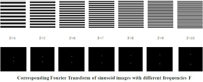
The next figures show the images of the sinusoid with various frequencies. It is highly seen that as the frequency of the sinusoid is increased, the distance between the two points corresponding to the frequency in the Fourier domain also increases. The points represent the transformation of the continuous signal to discrete signals upon undergoing Fourier Transform.

When a constant bias is added to the sinusoid, another peak located at the center between the two points. This is similar to a dirac-delta function centered at the middle of the two mirror imaged frequencies. In order to determine the peak frequencies, the 3D plot is performed.

The result of the Fourier Transform of the additional non-constant bias to the sinusoid is the appearance of other peaks that are located at the frequency values of the bias. Note that for every frequency, there are two peaks found because the Fourier transform consists of complex numbers, so the absolute value is taken. Thus, the negative and positive values are considered.

When the sinusoid is rotated, the corresponding Fourier transformed image is also rotated, the angle of which depends on the rotation angle of the input. This is observed from the figures below.

The next two figures are the image of the Fourier transform (right) of the product of two sinusoid running in X and Y axes.

The last four figures correspond to the addition of a non-constant bias at different rotation angles to the product of the two sinusoids above. The bias used in the first two images is a sinusoid with frequency F=20 and rotated to theta=60 degrees. The last two shows the image of the input sinusoid biased with another sinusoid at F=18 and theta=90degrees. It was predicted that another two points will appear on the FT and these are rotated in angles equal to the rotation angle used.

In this activity, I am giving myself a grade of 10 since all the tasks are completed and with desirable and correct results.

I would like to thank Gary Garcia and Winsome Rara for helping me improve my images.

Fourier Transform Model of Image Formation

Fourier Transform (FT) is the transformation of any input signal found in spatial domain into its frequency domain (1). For images, FT is used to decompose the each point into its corresponding sine or cosine components . However, images do not fully show all the frequencies composing the images. Thus, this activity is limited to the discrete Fourier Transform which shows limited number of frequencies but are enough to depict the spatial domain of the image.

In this activity, the Fourier Transform of different images are taken. Moreover, the properties and extension of Fourier Transform such as convolution and correlation are implemented.

The figures above describe the transformation of the original image (first image) as it undergoes FFT2 and FFTSHIFT. The third picture represents the Fourier transformed image which is a central bright spot. This agrees with the ideal Fourier transformation of circle. Applying another fourier transformation to the previously transformed image inverts the image with respect to the horizontal axis.

Applying the same procedure to letter "A", I arrived at the figures above. The inversion of "A" is still experience upon the application of another Fourier transform as shown in the last figure above. The star-like spread of light in the image just above the last image shows the fftshift of "A".

The figure above shows the effect of the size of the aperture to the quality of the image. Notice that as the aperture gets larger, the image's resolution becomes better.

For the images above, it can be seen that the sentence "The rain in Spain stays mainly in the plain" correlates with the letter "A" by producing more intense light in the part of the sentence which contains "A".

The Last three figures shows the corresponding image produced when an image pattern with a sum of zero is convolved with another image. It can be observed that some parts of the word "VIP" are lost depending on the location of the zeroed-sum in the matrix. The figures also show that the spot pattern gives out the best image quality among the three matrix patterns.

I would like to thank Master and Jaya for reminding me of the deadline of this activity as well as Gary and Rara for giving suggestions on improving my blog.

For this activity, I am giving myself a grade of 9. I was not able to attend the class and I finished the activity in a later time.

References:
1. http://homepages.inf.ed.ac.uk/rbf/HIPR2/fourier.htm

Enhancement by histogram manipulation

Not all images we capture have perfect contrast!... This is basically the motivation of this activity. Several techniques have been implemented in order to enhance images qualities. One of these is through histogram manipulation.
Histogram shows the pixel number in the image, each having one of the 256 possible values (1). The brightness of the images is shown in the histogram through the peaks in each pixel number. Histograms are manipulated by equalizing the distribution of the pixel numbers of the image. New brightness values are reassigned in the image's pixel numbers but the relationship among the pixel numbers are retained, that is, the pixels darker than other pixels still appear darker.

For this activity...

First thing I did: Find a grayscale image in the web. The chosen image is shown in Figure 1.
Reference:
http://images.google.com.ph/imgres?imgurl=http://www.atpm.com/13.02/images/ps-grayscale-4.jpg&imgrefurl=http://www.atpm.com/13.02/photoshop.shtml&usg=__ToqI_jVS80Y4k_ezF1QCq2TI03k=&h=280&w=420&sz=44&hl=tl&start=116&sig2=JetPq2CRGpzxKvLgJe0AMg&um=1&tbnid=lpf4uDD45kW5kM:&tbnh=83&tbnw=125&prev=/images%3Fq%3Dgrayscale%252Bblur%2Bimage%26ndsp%3D20%26hl%3Dtl%26client%3Dfirefox-a%26rls%3Dorg.mozilla:en-US:official%26sa%3DN%26start%3D100%26um%3D1&ei=pWFJSqCEF4_6kAXB67TwCQ

Figure 1. Original image

My main goal in this activity is to enhance the image above. To achieve this, I used Scilab and find the histogram of the image, the normalized probability distribution function (PDF) of the graylevel. Then, the PDF of the image is taken by simply dividing the frequencies by the total number of pixels of the image. The cumulative sum of the PDF is the Cumulative Distribution Function (CDF). Figures 2 and 3 show the histogram and CDF of the image, respectively.

Figure 2. Histogram of the image

Figure 3. CDF of the image

Each graylevel has a corresponding PDF value. In order to enhance the image, I created a desired CDF. In my case, I used the equation of a straight line. The figure below is my desired CDF.

Figure 4. Desired CDF

Each value in the image's CDF is then matched with the value of the desired CDF. I did this by looking for the y-values of the CDF of the image that are equal to the y-axis of the desired CDF and then getting the grayscale value of the desired CDF and put these in a new matrix having the same size as the image.
After reconstructing the image, I look for its corresponding histogram and CDF. The CDF of the new image must be in close relation with the desired CDF.

Figure 5. Collated results of the simulation

Code:
image=imread('act4 picture.jpg');
subplot(241)
imshow(image,[]);
//histogram
H=[];
counter=1;
for i = 0:255;
num=find(image==i);
H(counter)=length(num);
counter=counter+1;
end;
I=[1:256];//graylevel
subplot(242);
hist=plot(0:255,H);

//CDF of the image
tot=cumsum(H/length(image));
subplot(243);
cdf=plot(0:255,tot);

//desired CDF
j=[0:1:255];
slope=1/255;
line=slope*j;
subplot(244);
plot(j,line);

//mapping
s=size(image);
mat=spzeros(s(1),s(2));
for j=[1:length(I)];
mat=mat+round(bool2s(image==I(j))*tot(j)/slope);
end;

subplot(245);
imshow(mat,[]);

//histogram of the reconstructed image
new=[];
c=1;
for i = 0:255;
num2=find(mat==i);
new(c)=length(num2);
c=c+1;
end;
subplot(246);
hist2=plot(0:255,new);
//CDF of the new image
tot2=cumsum(new/length(mat));
subplot(247);
cdf2=plot(0:255,tot2);

The code was implemented to other images and these are the results.

Figure 6. The first three columns in the first row show the details of the original images, that is, the histogram and CDF. The fourth column is the desired CDF and the second row shows the reconstructed image with its corresponding histogram and CDF.

The human eyes respond to light in a nonlinear behavior. Thus, choosing a CDF that fits the behavior of the human eyes, logarithmic function [y=log(x)] is applicable. Replacing the desired CDF from a straight line into a logarithmic function, I arrived at the following results below.

Figure 7. left- original image; right- reconstructed image

It can be noticed from the reconstructed images still show good contrast but are brighter at some regions. This shows that the histograms of these reconstructed images are evenly distributed to the different gray levels, only that some gray level occurs more frequently than others at larger diffferences.

I would like to acknowledge Gary Carcia, Jica Monsanto and Jaya Combinido for helping me improve my code and giving constructive criticisms to my work.
I think I have performed all the tasks needed for this activity. So I am giving myself a grade of 10.

Additional Information:

I have found an article which performed image contrast enhancement based on the generalized histograms by relaxing the restriction of using the integer count. The abstract of the paper reads,

"We present an adaptive contrast enhancement method based on the generalized histogram, which is obtained by relaxing the restriction of using the integer count. For each pixel, the integer count 1 allocated to a pixel is split into the fractional count and the remainder count. The generalized histogram is generated by accumulating the fractional count for each intensity level and distributing the remainder count uniformly throughout the intensity levels. The intensity mapping function, which determines the contrast gain for each intensity level, is derived from the generalized histogram. Since only the fractional part of the count allocated to each pixel is
used for increasing the contrast gain of its intensity level, the amount of contrast enhancement is adjusted by varying the fractional count according to regional characteristics. The proposed
scheme produces visually more pleasing results than the conventional histogram equalization."

Title: Image contrast enhancement based on the generalized histogram
Authors: Byoung-Woo Yoon and Woo-Jin Song

References and Image url:
1. J. Russ, The Image Processing Handbook, Fifth Edition, CRC Press.
http://incisors.files.wordpress.com/2008/06/truecolor.jpg
http://www.dolphinsc.com/images/Dolphin.jpg